Root-Bracketing Quartile Algorithm
by
Namir C. Shammas
Numerical analysis offers a rich set of algorithms to solve for real roots of single nonlinear functions. The simplest class of root-seeking algorithms is the root-bracketing algorithms. These algorithms work by taking an interval that contains a root and zooming in on that root. The simplest, and slowest, root-seeking algorithm is the Bisection algorithm. This method works by selecting the middle of the interval and determining which half of the interval to discard. Each iteration reduces the root-hosting interval by half until the interval becomes small enough to contain the root within an accepted tolerance value.
The pseudo code for the Bisection method is:
Given: An interval [A, B] that contains a root for function f(X), such that f(A)*f(B) < 0.
The Bisection method is the slowest root-seeking method. However, since the method uses the sign of the targeted function, convergence is guaranteed if the initial conditions are true.
Another root-seeking algorithm is the method of False Position. It is more efficient than the Bisection method. The False Position algorithm looks at the function values at A and B as weights used to calculate the next guess. The following equation shows how to calculate the new guess:
M = (f(B) * A - f(A) * B) / (f(B) - f(A))
The algorithm performs a function sign test, just like with the Bisection algorithm, to determine which interval end is replaced by the new guess M. However, this method does not shrink the interval as one might expect. To stop iteration, an implementation of the method of False Position must compare the most two recent values M. Iteration resumes as long as the absolute difference of these values exceeds a tolerance value.
The new Quartile algorithm adopts a middle strategy regarding the use of the function values at A and B. The method compares the absolute values of f(A) and f(B) to determine how close to A or B the next guess for the root will be located.
Here is the pseudo code for Quartile algorithm:
Given: An interval [A, B] that contains a root for function f(X), such that f(A)*f(B) < 0.
The coefficient alpha can be in the range of 0.25 to 0.30. When the value for alpha is 0.5, the Quartile algorithm behaves just like the Bisection algorithm. Thus, conceptually, the Bisection method is a special case of the Quartile algorithm.
To compare the Bisection, Quartile, and False Position algorithms, consider the function f(x) = ex – 3x2 = 0 and tolerance = 1E-7. This function has roots near -0.459, 0.910, and 3.733. The following table shows the initial values for A and B, and the number of function calls for the Bisection, Quartile, and False Position algorithms. Comparing the Bisection and Quartile methods, the table shows that the Quartile algorithm requires fewer function calls to obtain a root in all the cases listed. Comparing the Quartile and False Position methods, the table shows the Quartile algorithm is no worse than the False Position in 6 (out of 10) cases.
| Initial A | Initial B | Bisection | Quartile | False Position |
| 3 | 4 | 26 | 17 | 14 |
| 3 | 5 | 27 | 20 | 41 |
| 3 | 6 | 27 | 19 | 93 |
| 2 | 5 | 27 | 20 | 46 |
| 0 | 1 | 26 | 19 | 9 |
| 0 | 2 | 27 | 19 | 18 |
| 0 | 3 | 27 | 22 | 12 |
| -1 | 0 | 26 | 21 | 16 |
| -2 | 0 | 27 | 20 | 29 |
| -3 | 0 | 27 | 20 | 42 |
Here is another example, using function f(x) = ln(x4) - x. In this case the False Position method performed better than the Quartile method, which in turn performed better than the Bisection method.
|
Initial A |
Initial B |
Bisection |
Quartile |
False Position |
|
3 |
9 |
28 |
18 |
8 |
|
4 |
9 |
28 |
22 |
8 |
|
5 |
9 |
28 |
21 |
8 |
|
6 |
9 |
27 |
19 |
8 |
|
7 |
9 |
27 |
18 |
8 |
|
8 |
9 |
26 |
22 |
7 |
|
8 |
10 |
27 |
18 |
9 |
|
8 |
11 |
27 |
21 |
10 |
|
8 |
12 |
28 |
21 |
11 |
|
8 |
13 |
28 |
21 |
11 |
|
8 |
14 |
28 |
21 |
12 |
|
8 |
15 |
29 |
21 |
13 |
A third example is the polynomial f(x) = (x - 10.1234)(x + 10.1234)(x - 3.4567)(x + 3.4567). In this case the False Position method performed better than the Quartile method (except for two cases), which in turn performed better than the Bisection method.
| Initial A | Initial B | Bisection | Quartile | False Position |
| 9 | 11 | 27 | 23 | 14 |
| 9 | 12 | 27 | 22 | 20 |
| 8 | 12 | 28 | 23 | 21 |
| 8 | 14 | 28 | 21 | 35 |
| 7 | 14 | 29 | 22 | 36 |
| 0 | 7 | 29 | 22 | 8 |
| 0 | 6 | 28 | 22 | 8 |
| 1 | 7 | 28 | 21 | 8 |
| 1 | 6 | 28 | 21 | 8 |
| 2 | 7 | 28 | 21 | 7 |
| 2 | 6 | 28 | 21 | 7 |
| 2 | 5 | 27 | 22 | 9 |
| 2 | 4 | 27 | 18 | 8 |
Here is the VBA source code for an Excel file that was used to test the first function. The code for the other functions differs in how Function F(X As Double) As Double is coded.
Option Explicit

Function F(X As Double) As Double
  F = Exp(X) - 3 * X ^ 2
End Function

Sub test()
  Const TOLER = 0.0000001
  Const ALPHA = 0.27
  Dim A As Double, B As Double, M As Double, LastM As Double
  Dim FA As Double, FB As Double, FM As Double
  Dim ColA As Integer, ColB As Integer, ColM As Integer
  Dim Row As Integer, Count As Integer

  Range("C2:Z1000").Clear

  Row = 2
  Do Until Cells(Row, 1) = ""

    ' Perform the Bisection Method
    ColA = 4
    ColB = 5
    ColM = 6

    A = Cells(Row, 1)
    B = Cells(Row, 2)

    FA = F(A)
    FB = F(B)
    Count = 2
    Do
      M = (A + B) / 2
      FM = F(M)
      Count = Count + 1
      If FM * FA > 0 Then
        A = M
        FA = FM
      Else
        B = M
        FB = FM
      End If
    Loop Until Abs(A - B) < TOLER

    Cells(Row, ColA - 1) = Count
    Cells(Row, ColA) = A
    Cells(Row, ColB) = B
    Cells(Row, ColM) = M
    Cells(Row, ColM + 1) = FM

    ' Perform the Quartile Method
    ColA = ColM + 3
    ColB = ColA + 1
    ColM = ColB + 1

    A = Cells(Row, 1)
    B = Cells(Row, 2)

    FA = F(A)
    FB = F(B)
    Count = 2
    Do
      If Abs(FA) < Abs(FB) Then
        M = A + ALPHA * (B - A)
      Else
        M = A + (1 - ALPHA) * (B - A)
      End If
      FM = F(M)
      Count = Count + 1
      If FM * FA > 0 Then
        A = M
        FA = FM
      Else
        B = M
        FB = FM
      End If
    Loop Until Abs(A - B) < TOLER

    Cells(Row, ColA - 1) = Count
    Cells(Row, ColA) = A
    Cells(Row, ColB) = B
    Cells(Row, ColM) = M
    Cells(Row, ColM + 1) = FM

    ' Perform the False Position Method
    ColA = ColM + 3
    ColB = ColA + 1
    ColM = ColB + 1

    A = Cells(Row, 1)
    B = Cells(Row, 2)

    FA = F(A)
    FB = F(B)
    M = A
    Count = 2
    Do
      LastM = M
      M = (FB * A - FA * B) / (FB - FA)
      FM = F(M)
      Count = Count + 1
      If FM * FA > 0 Then
        A = M
        FA = FM
      Else
        B = M
        FB = FM
      End If
    Loop Until (Abs(M - LastM) < TOLER) Or (FA = FB)

    Cells(Row, ColA - 1) = Count
    Cells(Row, ColA) = A
    Cells(Row, ColB) = B
    Cells(Row, ColM) = M
    Cells(Row, ColM + 1) = FM

    Row = Row + 1
  Loop

End Sub
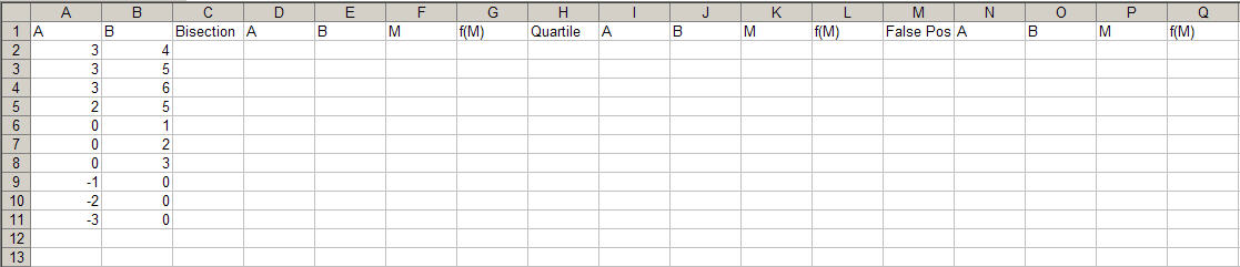
The following figure shows the Excel sheet with initial data and column headings:
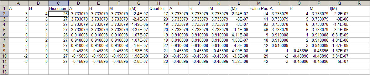
Notice that columns 1 and 2 (from row 2 and down) contain different sets of initial values for the interval [A, B]. Here is a figure showing the output that was generated by the above VBA code:
While root-bracketing algorithms are not the fastest root-seeking methods, you can still use them as a backup in conjunction with faster algorithms like Newton's method. The basic technique of using these double algorithms is to test if the new guess (generated by Newton's method or other efficient algorithms) falls outside a root-hosting interval. If this condition is true, then the root-bracketing algorithm kicks in and provides a better new guess for the root.
Copyright (c) Namir Shammas. All rights reserved.