New Root-Seeking Algorithms

by

Namir C. Shammas

This article presents a pair of new root-seeking algorithms that use an innovative approach. Testing these algorithms shows that they can reach a good approximation to the root in less iterations and/or fewer function calls than Newton’s method.

Overview of Newton’s Method

Newton’s method starts with a guess for the root and iterates to refine that guess. Each iteration requires the calculations of the function and the slope at the current guess, and yields a new guess for the root. The algorithm discards the older guesses. Typically, the value of the slope is approximated by a finite difference method. Thus, each iteration in Newton’s method requires two function calls. Other algorithms that diverge at a faster rate use approximations to higher derivatives and thus make more function calls per iteration in order to approximate the higher derivatives. In the majority of the root-seeking methods, that do not bracket the root, the iterations refine the guess for the root until it converges to an acceptable value that is close enough to the actual root.

To solve for:

f(X^*) = 0

Newton’s algorithm uses the following equation to refine the guess for the root:

X₁ = X₀ – f(X₀) / f’(X₀)

Where f’(X) is the derivative of f(X) with respect to X. You can evaluate an approximation to the derivative using, among others, the following equation:

f’(X) = [f(X + h) – f(X)] / h

Where h is a small increment and can be estimated as:

h = 0.01 * (|X| + 1)

Probing Algorithms

The two new algorithms that I designed share a common approach, yet differ in the details of their execution. The basic idea is to start with an initial guess which becomes a fixed vantage point. From this vantage point, the algorithm uses probes to find the root. Each probe generates a new value for the variable X and its corresponding function value. This function value gives an assessment of how good the probed value of X is. The iterations of the probing algorithms strive to obtain better probed values. During the iterations, the initial guess remains fixed.

Here is the abstract version of the probing algorithms:

1.       Given an initial guess X₀.

2.       Initialize an array of N probes. For each probe obtain a new value of X(i) and f(X(i)).

3.       Repeat the next steps

a.       Use the current array of N probes to interpolate a new probe value X(N+1) and its function value f(X(N+1)).

b.      Sort the array of the N+1 probe elements using the absolute value of f(X) as the sort key. This step places the best probe at the array index 1. Likewise, the worst probe appears at the array index N+1.

c.       If the probes show that the convergence criteria have been met, resume in step 4. Otherwise, perform another loop iteration.

4.       The best guess for the root is X(1)

The Probing Slopes Algorithm

The first variant of the probing algorithms attempts to find the critical slope that would zoom in on the root. In other words, the algorithm attempts to find the slope of the straight line connecting the initial guess point with the root. The initial guess point is (X₀,f(X₀)),where initial guess X₀. The root point is (X^*,0). The critical straight line passing through these two points is:

Critical slope = (f(X₀) – 0) / (X₀ – X*)

Calculating the critical slope is not possible since we do not know the value of the root, X*. The algorithm starts by calculating an array of three slopes, using the following equations:

S(1) =  [f(X + h) – f(X)] / h

S(2) = (1 + r)  S(1)

S(3) = (1 – r)  S(1)

Where r is a small number like 0.15 and  0.10. Notice that calculating the values for slopes S(2) and S(3) does not require evaluating the function f(x).

The algorithm uses the array of slopes to calculate the array of probed root values. The algorithm uses the following equation:

X(i) = X₀ – f(X₀) / S(i), for I = 1,2, and 3

Next, the algorithm calculates the array of function values Fx(i) = f(X(i)).

The steps up till now supply the algorithm with its initial probes. Each one of the three probes is made up of the values of a slope S(i), probed root value X(i), and probed function value Fx(i). Armed with the probes the algorithm starts its main loop. Each loop iteration performs the following tasks:

1.       Interpolate the first three elements of arrays S() and Fx() to calculate the slope S(4) for when the function value is 0. The calculated slope is designated as S(4) and represents a new element of the array of slopes S().

2.       Calculate the probed root value, X(4) = X₀ – f(X₀) / S(4), and then the probed function value, Fx(4) = f(X(4)).

3.       Sort the four-element arrays S(), X(), and Fx() using the absolute values of array Fx() as the sorting key. When the sorting step ends, the array elements at index 1 represent the best probe for the root. The array elements at index 4 represent the worst probe for the root.

The above loop ends when |X(1) – X(2)| fall below an acceptable tolerance limit. You can also use compare the absolute value of Fx(1) with a function tolerance value to stop the iterations. If the convergence conditions fail, the next iteration occurs. Since task 1 uses the first three elements of arrays S(), X(), and Fx(), the values of the elements at index 4 are ignored. In fact, tasks1 and 2 overwrite these values. As you can see in task 2, the algorithm retains the value of the initial guess X₀. Why retain this value and not update it with the value of X(1)? The answer lies with the fact that replacing X₀ with a new value requires calculating a new set of values for S(1), S(2), S(3), X(1), X(2), X(3), Fx(1), Fx(2), and Fx(3). Calculating these values comes at a price of making more evaluations of function f(X). This rise in the number of function evaluation makes the algorithm less efficient than Newton’s algorithm. By keeping the original guess for the root, the algorithm economizes on the number of invocation of f(x) without compromising on the speed of convergence. Since each iteration in the main loop requires only one invocation of f(x), compared to two for Newton’s method, the Probing Slopes Algorithm tends has an advantage. Using an efficient interpolation method, like the Lagrangian interpolation, adds to the overall efficiency of the implementation of the algorithm. Thus, the Probing Slopes Algorithm gains more advantage over Newton’s method.

The Probing Steps Algorithm

The second variant of the probing algorithms attempts to find the critical step that would zoom in on the root in one swoop. Of course, such a magical step does not exist. Instead, we can modify the Probing Slopes Algorithm to work with steps of X instead of function slopes.

Calculating the critical step is not possible since we do not know the value of the root, X*. The algorithm starts by calculating an array of three steps, using the following equations:

St(1) =  h * f(x) / [f(X + h) – f(X)]

St(2) = (1 + r) St(1)

St(3) = (1 – r) St(1)

Where r is a small number like 0.15 and 0.1. Notice that calculating the values for steps St(2) and St(3) does not require evaluating the function f(x).

The algorithm uses the array of slopes to calculate the array of probed root values. The algorithm uses the following equation:

X(i) = X₀ - St(i), for I = 1,2, and 3

Next, the algorithm calculates the array of function values Fx(i) = f(X(i)).

The steps up till now supply the algorithm with its initial probes. Each one of the three probes is made up of the values of a step St(i), probed root value X(i), and probed function value Fx(i). Armed with the probes the algorithm starts its main loop. Each loop iteration performs the following tasks:

1.       Interpolate the first three elements of arrays St() and Fx() to calculate the step St(4) for when the function value is 0. The calculated step is designated as St(4) and represents a new element of the array of steps St().

2.       Calculate the probed root value, X(4) = X₀ – St(4), and then the probed function value, Fx(4) = f(X(4)).

3.       Sort the four-element arrays St(), X(), and Fx() using the absolute values of array Fx() as the sorting key. When the sorting step ends, the values at index 1 represent the best probe for the root. The values at index 4 represent the worst probe for the root.

The above loop ends when |X(1)-X(2)| fall below an acceptable tolerance limit. You can also use compare the absolute value of Fx(1) with a function tolerance value to stop the iterations. If the convergence conditions fail, the next iteration occurs. Since task number 1 uses the first three elements of arrays St(), X(), and Fx(), the values of the elements at index 4 are not used. In fact, tasks1 and 2 overwrite these values. As you can see in task 2, the algorithm retains the value of the initial guess X₀, for the same reason as the Probing Slopes Algorithm.

Testing the Probing Slopes Algorithm

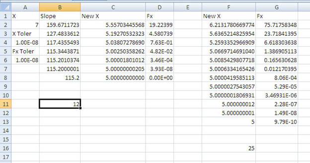
This section presents the tests results that compare the Probing Slopes Algorithm with Newton’s method. The test uses an Excel spreadsheet that has the following visual interface:

The VBA code used for this test is:

Option Explicit

Function F(X As Double) As Double

  F = Exp(X) - 3 * X ^ 2

End Function

Sub RootByCriticalSlopes()

  Const NUM_SLOPES = 3

  Const SLOPE_FACTOR = 0.15

  Dim XToler As Double, FxToler As Double

  Dim R As Integer, NumCalls As Integer

  Dim X As Double, S(NUM_SLOPES + 1) As Double

  Dim Fx(NUM_SLOPES + 1) As Double

  Dim Xnew(NUM_SLOPES + 1) As Double, Xold As Double

  Dim I As Integer, J As Integer

  Dim Sum As Double, Prod As Double, FxVal As Double, Diff As Double

  Dim h As Double, Buff As Double

  ' Probing slopes algorithm

  X = Cells(2, 1)

  XToler = Cells(4, 1)

  FxToler = Cells(6, 1)

  R = 2

  FxVal = F(X)

  NumCalls = 1

  Range("B2:Z10000").Value = ""

  h = 0.01 * (1 + Abs(X))

  S(1) = (F(X + h) - FxVal) / h

  NumCalls = NumCalls + 1

  S(2) = S(1) * (1 + SLOPE_FACTOR)

  S(3) = S(1) * (1 - SLOPE_FACTOR)

  For I = 1 To 3

    Xnew(I) = X - FxVal / S(I)

    Fx(I) = F(Xnew(I))

    NumCalls = NumCalls + 1

  Next I

  Do

    Sum = 0

    For I = 1 To NUM_SLOPES

      Prod = S(I)

      For J = 1 To NUM_SLOPES

        If I <> J Then

          Prod = Prod * (0 - Fx(J)) / (Fx(I) - Fx(J))

        End If

      Next J

      Sum = Sum + Prod

    Next I

    S(4) = Sum

    Xnew(4) = X - FxVal / S(4)

    Cells(R, 2) = S(4)

    Cells(R, 3) = Xnew(4)

    Fx(4) = F(Xnew(4))

    NumCalls = NumCalls + 1

    Cells(R, 4) = Fx(4)

    R = R + 1

    ' remove worst fx() value

    For I = 1 To NUM_SLOPES

      For J = I + 1 To NUM_SLOPES + 1

        If Abs(Fx(I)) > Abs(Fx(J)) Then

          Buff = Fx(I)

          Fx(I) = Fx(J)

          Fx(J) = Buff

          Buff = S(I)

          S(I) = S(J)

          S(J) = Buff

          Buff = Xnew(I)

          Xnew(I) = Xnew(J)

          Xnew(J) = Buff

        End If

      Next J

    Next I

  Loop Until Abs(Xnew(1) - Xnew(2)) <= XToler Or Abs(Fx(1)) <= FxToler

  Cells(R + 2, 2) = NumCalls

  ' now test Newton's method

  X = Cells(2, 1)

  FxVal = F(X)

  R = 2

  NumCalls = 1

  Do

    h = 0.01 * (1 + Abs(X))

    Diff = h * FxVal / (F(X + h) - FxVal)

    NumCalls = NumCalls + 1

    X = X - Diff

    FxVal = F(X)

    NumCalls = NumCalls + 1

    Cells(R, 6) = X

    Cells(R, 7) = FxVal

    R = R + 1

  Loop Until Abs(Diff) <= XToler Or Abs(FxVal) < FxToler

  Cells(R + 2, 6) = NumCalls 

End Sub

The above code shows the function F which contains a sample test f(x) function. The code for function F changes as the test function f(x) changes.

The Function f(x)=Exp(x)-3*X^2

The first test function is f(X) = Exp(X)-3^X2. The following figure shows a graph for this function.

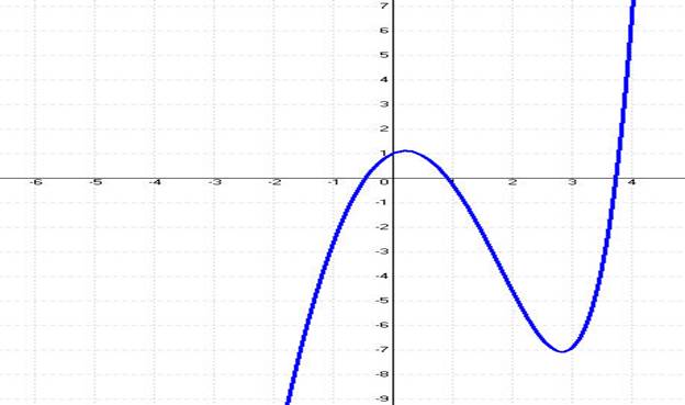
Table 1. Test results for f(X)=Exp(X)-3*X^2 for Xtoler =1E-8 and FxToler = 1E-8.

Table 1 shows the results for function f(X) = e^X – 3X² for X tolerance of 1E-8 and function tolerance of 1E-8. The table shows a set of initial guesses supplied to the VBA subroutine RootByProbingSlopes.  The tested function has three roots near 3.733, 0.9100, and -0.4589. The table shows that for each initial guess, the Probing Slopes Algorithm required less iterations and functions calls than Newton’s method.

The Function f(X) = exp(-X) – exp(-3)

The second function is f(X) = = exp(-X) – exp(-3) whose graph appears in the next figure:

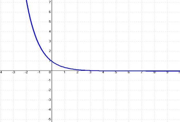
Table 2. Test results for f(X)=Exp(-X)- Exp(-3) for Xtoler =1E-8 and FxToler = 1E-8.

Table 2 shows the results for function f(X) = e-^X – e-³ for X tolerance of 1E-8 and function tolerance of 1E-8. The table shows a set of initial guesses supplied to the VBA subroutine RootByProbingSlopes.  The tested function has a root of 3. The table shows that for each initial guess below the root value, the Probing Slopes Algorithm required less iterations and functions calls than Newton’s method. The value of X = 6 is an exception since Newton’s method required 2 iterations less, but made 16 additional function calls.

The Test Polynomial

The third test function is:

f(X) = 0.005 * (X+5) * (X+3) * (X+1) * (X-5) * (X-3) * (X-1)

Which has The following figure shows a graph of the test polynomial.

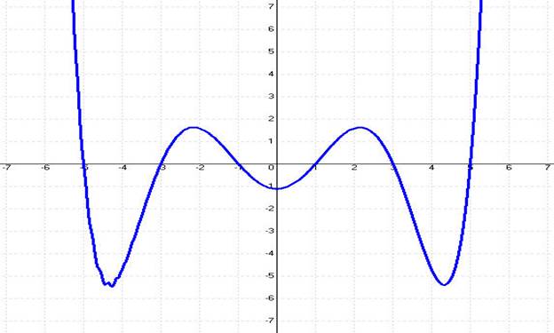
Table 3. Test results for f(X) = 0.005 * (X+5) * (X+3) * (X+1) * (X-5) * (X-3) * (X-1) for Xtoler =1E-8 and FxToler = 1E-8.

Table 3 shows the results for the test polynomial for X tolerance of 1E-8 and function tolerance of 1E-8. The table shows a set of initial guesses supplied to the VBA subroutine RootByProbingSlopes.  The tested function has roots at 5, 3, 1, -1, -3, and -5.  The table shows that for each initial guess below the root value, the Probing Slopes Algorithm required less iterations and functions calls than Newton’s method. The value of X = 0 is an exception since both algorithms required the same number of iterations to reach the root of 5.

Testing the Probing Steps Algorithm

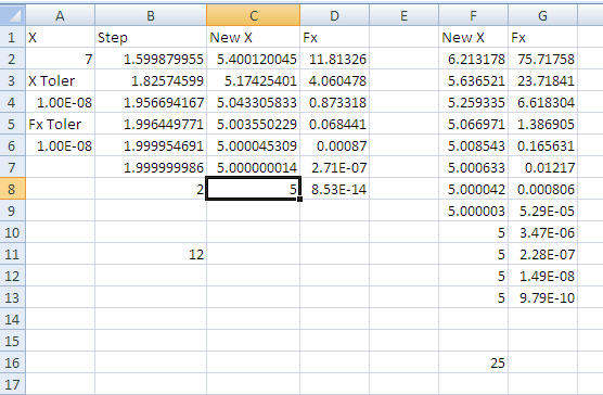
This section presents the tests results that compare the Probing Steps Algorithm with Newton’s method. The test uses an Excel spreadsheet that has the following visual interface:

The VBA code used for this test is:

Option Explicit

Function F(X As Double) As Double

  F = Exp(X) - 3 * X ^ 2

End Function

Sub RootByProbingSteps()

  Const NUM_STEPS = 3

  Const SLOPE_SHIFT = 5

  Const STEP_FACTOR = 0.15

  Dim XToler As Double, FxToler As Double

  Dim R As Integer, NumCalls As Integer

  Dim X As Double, St(NUM_STEPS + 1) As Double, Fx(NUM_STEPS + 1) As Double

  Dim Xnew(NUM_STEPS + 1) As Double, Xold As Double

  Dim I As Integer, J As Integer

  Dim Sum As Double, Prod As Double, FxVal As Double, Diff As Double

  Dim h As Double, Buff As Double

  X = Cells(2, 1)

  XToler = Cells(4, 1)

  FxToler = Cells(6, 1)

  Range("B2:Z10000").Value = ""

  R = 2

  FxVal = F(X)

  NumCalls = 1

  h = 0.01 * (1 + Abs(X))

  St(1) = h * FxVal / (F(X + h) - FxVal)

  NumCalls = NumCalls + 1

  St(2) = St(1) * (1 + STEP_FACTOR)

  St(3) = St(1) * (1 - STEP_FACTOR)

  For I = 1 To 3

    Xnew(I) = X - St(I)

    Fx(I) = F(Xnew(I))

    NumCalls = NumCalls + 1

  Next I

  Do

    Sum = 0

    For I = 1 To NUM_STEPS

      Prod = St(I)

      For J = 1 To NUM_STEPS

        If I <> J Then

          Prod = Prod * (0 - Fx(J)) / (Fx(I) - Fx(J))

        End If

      Next J

      Sum = Sum + Prod

    Next I

    St(4) = Sum

    Xnew(4) = X - St(4)

    Cells(R, 2) = St(4)

    Cells(R, 3) = Xnew(4)

    Fx(4) = F(Xnew(4))

    NumCalls = NumCalls + 1

    Cells(R, 4) = Fx(4)

    ' remove worst fx() value

    For I = 1 To NUM_STEPS

      For J = I + 1 To NUM_STEPS + 1

        If Abs(Fx(I)) > Abs(Fx(J)) Then

          Buff = Fx(I)

          Fx(I) = Fx(J)

          Fx(J) = Buff

          Buff = St(I)

          St(I) = St(J)

          St(J) = Buff

          Buff = Xnew(I)

          Xnew(I) = Xnew(J)

          Xnew(J) = Buff

        End If

      Next J

    Next I

    R = R + 1

  Loop Until Abs(Xnew(1) - Xnew(2)) <= XToler Or Abs(Fx(1)) <= FxToler

  Cells(R + 2, 2) = NumCalls

  ' now test Newton's method

  X = Cells(2, 1)

  FxVal = F(X)

  R = 2

  NumCalls = 1

  Do

    h = 0.01 * (1 + Abs(X))

    Diff = h * FxVal / (F(X + h) - FxVal)

    NumCalls = NumCalls + 1

    X = X - Diff

    FxVal = F(X)

    NumCalls = NumCalls + 1

    Cells(R, 6) = X

    Cells(R, 7) = FxVal

    R = R + 1

  Loop Until Abs(Diff) <= XToler Or Abs(FxVal) < FxToler

  Cells(R + 2, 6) = NumCalls

End Sub

The above code shows the function F which contains a sample test f(x) function. The code for function F changes as the test function f(x) changes.

The Function f(x)=Exp(x)-3*X^2

The first test function is f(X) = Exp(X)-3^X2. The following figure shows a graph for this function.

Table 41. Test results for f(X)=Exp(X)-3*X^2 for Xtoler =1E-8 and FxToler = 1E-8.

Table 4 shows the results for function f(X) = e^X – 3X² for X tolerance of 1E-8 and function tolerance of 1E-8. The table shows a set of initial guesses supplied to the VBA subroutine RootByProbingSteps.  The tested function has three roots near 3.733, 0.9100, and -0.4589. The table shows that for each initial guess, the Probing Steps Algorithm required less iterations and functions calls than Newton’s method.

The Function f(X) = exp(-X) – exp(-3)

The second function is f(X) = = exp(-X) – exp(-3) whose graph appears in the next figure:

Table 5. Test results for f(X)=Exp(-X)- Exp(-3) for Xtoler =1E-8 and FxToler = 1E-8.

Table 5 shows the results for function f(X) = e-^X – e-³ for X tolerance of 1E-8 and function tolerance of 1E-8. The table shows a set of initial guesses supplied to the VBA subroutine RootByProbingSteps.  The tested function has a root of 3. The table shows that for each initial guess below the root value, the Probing Slteps Algorithm required less iterations and functions calls than Newton’s method. The value of X = 6 is an exception since Newton’s method required the same number of iterations, but made 18 additional function calls.

The Test Polynomial

The third test function is:

f(X) = 0.005 * (X+5) * (X+3) * (X+1) * (X-5) * (X-3) * (X-1)

Table 6. Test results for f(X) = 0.005 * (X+5) * (X+3) * (X+1) * (X-5) * (X-3) * (X-1) for Xtoler =1E-8 and FxToler = 1E-8.

Table 6 shows the results for the test polynomial for X tolerance of 1E-8 and function tolerance of 1E-8. The table shows a set of initial guesses supplied to the VBA subroutine RootByProbingSteps.  The tested function has roots at 5, 3, 1, -1, -3, and -5.  The table shows that for each initial guess below the root value, the Probing Slope Algorithm required less iterations and functions calls than Newton’s method.

Conclusions

The Probing Slopes Algorithm and the Probing Steps Algorithms demonstrated in the three examples that they outperform Newton’s method. The tests also show that the Probing Steps Algorithm slightly outperforms the Probing Slopes Algorithm. The recommendation is to use the Probing Steps Algorithm, with the Probing Slopes Algorithm as plan B.

Back to menu

Copyright (c) Namir Shammas. All rights reserved.